Free supercomputing for research: A tutorial on using Python on the Open Science Grid
January 03, 2017
Supercomputing resources typically cost money, but the Open Science Grid (OSG) provides high-throughput computing to any researcher in the US for free. Briefly, OSG users can run jobs on servers owned by dozens of academic institutions, whenever those servers are not actively running a job for its owners.
Besides cost, a second major barrier to entry for those who are new to supercomputing (or, specifically, Condor) is the necessary troubleshooting before we can actually run our jobs. The purpose of this tutorial is to provide a complete example for running Python jobs on the OSG. This example is nontrivial, in that it includes multiple data sets, public libraries (e.g. scipy), private libraries, and analyzing output. In complement to this tutorial, the OSG has tutorials, a structured class, and extremely helpful online support when you get stuck.
This tutorial goes through the steps of manually connecting to and running commands on the remote server, but see the Fabfile section at the bottom for how this can be automated on your local machine.
Step 1. Register with OSG
Sign up for an account at osgconnect.net. If someone in your lab has not already started a project on OSG connect, start one here. For more help on these steps, see the OSG tutorials here. This may take a few hours or days to get approved.
Step 2. Install necessary programs.
On Windows, you need PuTTY in order to remotely log into the OSG servers. Also install WinSCP, which allows you to transfer files between your local machine and the OSG system.
On Mac, I believe the equivalent programs are Terminal and Cyberduck.
Step 3. Remotely access the OSG system
This step is written for Windows, but the steps should be similar on Mac. Alternatively, google “SSH on Mac.”
Using PuTTY, enter the following information:
- Hostname: login.osgconnect.net
- Port: 22
- Connection Type: SSH
A command window should then appear. When prompted “login as: “ enter the username you made for OSG connect. You will then be prompted for the password you made. You should then be on an OSG server! We will call this server the submit server because it is the computer on which we will submit our job. In contrast, the job servers are the computers on which our Python code actually runs, but we never interface directly with these servers.
If you have not used a Linux terminal before, I would recommend this tutorial on the commands to navigate the terminal and manipulate files.
Step 4. Download this tutorial
The files for this tutorial are located on GitHub here. I will describe each of these files in the steps below, when they become relevant.
Clone these files into your home directory on the OSG system, and then navigate into the folder created.
$ git clone https://github.com/srcole/demo_OSG_python
$ cd demo_OSG_python/
There are some unnecessary files you can remove to reduce clutter.
$ rm LICENSE
$ rm -rf .git
Step 5. Create the Python virtual environment
In high-throughput computing, we are running our code on many servers, and we want to assure that the Python environment is exactly the same on all of these machines. Therefore, on the submit server, we first create a Python virtual environment which will be installed on each machine on which we run Python code.
The bash script, create_virtenv.sh, was written to create this virtual environment. It loads Python 2.7 and several libraries (e.g. numpy), and then compresses this virtual environment. The first command below is needed in order to give you permission to execute create_virtenv.sh. The second command actually creates the virtual environment, and will take several minutes.
$ chmod +x create_virtenv.sh
$ ./create_virtenv.sh
After the virtual environment is created, the file python_virtenv_demo.tar.gz will appear in the local directory. Remove the (uncompressed) folder because it is no longer needed:
$ rm -R python_virtenv_demo
In this case, the virtual environment includes numpy, scipy, scikit-learn, matplotlib, h5py, and pandas. While not all of these libraries are necessary for this tutorial, I have kept them in because I need them for my project. Adding these libraries often resulted in Python ImportErrors that were only solved by loading nonobvious modules in exe_find_PsTs.sh and adding requirements to sub_PsTs.submit. You may run into more ImportErrors when working with other libraries. In that case, open a ticket with the osgconnect support team, and they will help you.
Step 6. Transfer input data to Stash
In the OSG network, data is stored in the Stash directory. Therefore, we move the data set that we want to analyze to the Stash. In the command below, replace USERID with your OSG connect username.
$ mv lfp_set/ /stash/user/USERID/lfp_set/
Step 7. Compress personal libraries
This job requires my personal library for analyzing the waveform shape of oscillations, misshapen. A static version was included in the demo folder because it cannot be pip-installed like numpy.
We need to compress this library in order to transport it to the job servers. We then remove the uncompressed folder.
$ tar -cvzf misshapen.tar.gz misshapen
$ rm -R misshapen
Step 8. Submit jobs to run python script
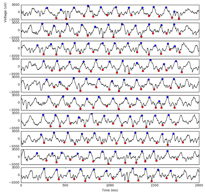
We are almost ready to actually run the analysis script, find_PsTs.py. This script uses the public libraries in the virtual environment, the misshapen library from the previous step, and the util.py library also included among the demo files. It is a simple script that finds the peaks and troughs of an oscillation in a time series (see the output figure below). We want 10 job servers to each import 1 time series and output two numpy files (.npy) containing the samples at which peaks and troughs are located.
The executable file exe_find_PsTs is the bash script that is run on each of the job servers. It does the following:
- Loads the Python virtual environment
- Imports the data from the Stash using StashCache
- Decompresses any personal libraries (misshapen)
- Run the python analysis script, find_PsTs.py
- Compresses output files generated by the python script.
First, we need to make a directory for the log files, which contain information about how the job was run and if there were any errors and printed output.
$ mkdir Log
We are now ready to submit our job. We do this by submitting a “submit file,” which in this case is sub_PsTs.submit. This submit file contains information including:
- Name of the bash script to execute
- Files to be transferred to the job servers
- Locations to save log files
- Hardware specifications for job servers (# CPUs, Memory, and Disk)
- Software specifications for job servers (has necessary modules)
- How many processes are run. In this case, we run 10 processes, which correspond to the input files 0.npy, 1.npy, … 9.npy.
$ condor_submit sub_PsTs.submit
For more information on submit files, see this documentation.
We can watch the progress of our jobs using the ‘watch command’, which will update every 2 seconds in this case. Replace USERID with your OSG connect username.
$ watch -n2 condor_q USERID
Each job should take less than a minute to run, but this is variable since it depends on the speed of the specific servers that are analyzing the data. After some jobs are complete, get out of this watch by pressing CTRL+C. You can then navigate to the Log directory and read the .error, .log, and .out files in order to see if they ran correctly.
NOTE: Currently, jobs occasionally run into errors. However, these jobs will usually run fine after resubmitting. I opened a ticket open on osgconnect.net to try to get rid of this occasional issue.
Step 9. Transfer output files from the OSG system to your local machine.
Access the OSG system with WinSCP using the same information and credentials used for PuTTY in Step 3. This GUI will allow you to copy the output files (e.g. out.29213003.0.tar.gz) to your local machine. On your local machine, you can decompress these files and confirm that your job ran correctly by plotting the input time series with the computed peak and trough samples. I did this in this notebook and obtained the plot below.
UPDATE: Fabfile
After I initially posted this tutorial, someone suggested using the python library, Fabric. With a Fabric fabfile, we can execute all of these commands on the OSG server with a single call of a python script from the command line on our local machine. Additionally, fabfile facilitates transferring files between local and remote servers. See the fabfile documentation for more information.
You can download the fabfile to run this demo here. You will just need to change the username input. Then navigate to the folder containing the fabfile in a command window and execute fab run_demo. The command prompt will then print your progress on the commands that are executing on the remote server. At the end, it will display where the output files have been downloaded.
Concluding notes
I hope you found this tutorial useful and easy to follow. If you ran into any issues, please contact me, and I will update this post.
I also hope you are motivated to utilize the OSG for your research supercomputing needs. It truly is a tremendous resource. If you’re interested in learning more, I would highly recommend their summer school which will give you much more intimate knowledge for using the OSG (also, it’s a completely free! Even travel expenses are covered.) But if you don’t want to do that, then check out their aforementioned resources.
I would like to thank Dr. Bala Desinghu at the University of Chicago for his amazing support for helping to get my jobs to run properly and finding solutions to bypass the many Python ImportErrors.